Cell-Cell Interaction Analysis with Xenium Data
This tutorial runs through stLearn CCI analysis on extremely large data, containing >166,000 single cells with gene expression measured in space.
To increase computation speed, we grid the cells and perform stLearn CCI analysis while taking into account the proportion of different cell types detected per grid.
Environment setup
[1]:
import matplotlib.pyplot as plt
import stlearn as st
import pathlib as pathlib

st.settings.set_figure_params(dpi=120)

# Ignore all warnings
import warnings

warnings.filterwarnings("ignore")
/Users/andrew/conda/stlearn/lib/python3.10/site-packages/louvain/__init__.py:54: UserWarning: pkg_resources is deprecated as an API. See https://setuptools.pypa.io/en/latest/pkg_resources.html. The pkg_resources package is slated for removal as early as 2025-11-30. Refrain from using this package or pin to Setuptools<81.
  from pkg_resources import get_distribution, DistributionNotFound
/Users/andrew/conda/stlearn/lib/python3.10/site-packages/stlearn/tl/cci/het.py:206: NumbaDeprecationWarning: The keyword argument 'nopython=False' was supplied. From Numba 0.59.0 the default is being changed to True and use of 'nopython=False' will raise a warning as the argument will have no effect. See https://numba.readthedocs.io/en/stable/reference/deprecation.html#deprecation-of-object-mode-fall-back-behaviour-when-using-jit for details.
  @jit(parallel=True, nopython=False)
Loading the data
For this tutorial purpose, we don’t perform the clustering. Please run the clustering method with the clustering tutorial or a part of spatial trajectory inference tutorial.
[2]:
# Setup download directory and get data
st.settings.datasetdir =  pathlib.Path.cwd().parent / "data"
library_id = "Xenium_FFPE_Human_Breast_Cancer_Rep1"
data_dir = st.settings.datasetdir / "Xenium_FFPE_Human_Breast_Cancer_Rep1"
[3]:
st.datasets.xenium_sge(library_id=library_id, include_hires_tiff=True)
[4]:
adata = st.ReadXenium(feature_cell_matrix_file=data_dir / "cell_feature_matrix.h5",
                      cell_summary_file=data_dir / "cells.csv.gz",
                      library_id=library_id,
                      image_path=data_dir / "he_image.ome.tif",
                      scale=1,
                      spot_diameter_fullres=15,
                      alignment_matrix_file=data_dir / "he_imagealignment.csv",
                      experiment_xenium_file=data_dir / "experiment.xenium",
                      )
Added tissue image to the object!
[5]:
# QC - Filter genes and cells with at least 10 counts
st.pp.filter_genes(adata, min_counts=10)
st.pp.filter_cells(adata, min_counts=10)
[6]:
adata.X.toarray()
[6]:
array([[0., 0., 0., ..., 0., 0., 0.],
       [0., 0., 1., ..., 0., 0., 0.],
       [0., 0., 0., ..., 0., 0., 0.],
       ...,
       [4., 1., 5., ..., 0., 0., 3.],
       [1., 0., 0., ..., 0., 0., 0.],
       [4., 1., 3., ..., 0., 0., 0.]], dtype=float32)
[7]:
# Store the raw data for using PSTS
adata.raw = adata
[8]:
# Run PCA, neighbors and clustering.
st.em.run_pca(adata, n_comps=50, random_state=0)
st.pp.neighbors(adata, n_neighbors=25, use_rep='X_pca', random_state=0)
st.tl.clustering.louvain(adata, random_state=0)
OMP: Info #276: omp_set_nested routine deprecated, please use omp_set_max_active_levels instead.
PCA is done! Generated in adata.obsm['X_pca'], adata.uns['pca'] and adata.varm['PCs']
Created k-Nearest-Neighbor graph in adata.uns['neighbors']
Applying Louvain cluster ...
Louvain cluster is done! The labels are stored in adata.obs['louvain']
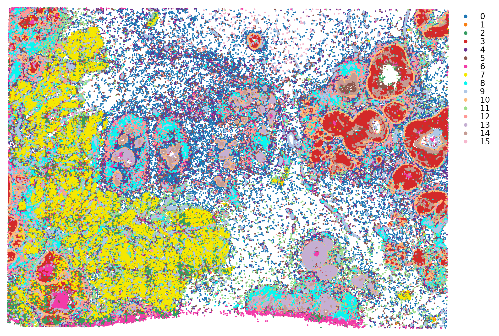
[9]:
st.pl.cluster_plot(adata, use_label="louvain", image_alpha=0, size=4, figsize=(10, 10))
[9]:
AnnData object with n_obs × n_vars = 164000 × 313
    obs: 'imagecol', 'imagerow', 'n_counts', 'louvain'
    var: 'gene_ids', 'feature_types', 'genome', 'n_counts'
    uns: 'spatial', 'pca', 'neighbors', 'louvain', 'louvain_colors'
    obsm: 'spatial', 'X_pca'
    varm: 'PCs'
    obsp: 'distances', 'connectivities'
Note on normalisation
No log1p or shrinking to make genes of similar expression range. In our case, for calling hotspots, we want genes to be more separate, since we select background genes with similar expression levels to detect hotspots.
[10]:
#### Normalize total...
st.pp.normalize_total(adata)
Normalization step is finished in adata.X
[11]:
adata.X.toarray()
[11]:
array([[0.        , 0.        , 0.        , ..., 0.        , 0.        ,
        0.        ],
       [0.        , 0.        , 1.787234  , ..., 0.        , 0.        ,
        0.        ],
       [0.        , 0.        , 0.        , ..., 0.        , 0.        ,
        0.        ],
       ...,
       [1.6926951 , 0.4231738 , 2.115869  , ..., 0.        , 0.        ,
        1.2695214 ],
       [1.4358974 , 0.        , 0.        , ..., 0.        , 0.        ,
        0.        ],
       [1.7777778 , 0.44444445, 1.3333334 , ..., 0.        , 0.        ,
        0.        ]], dtype=float32)
Gridding
Now performing the gridding. The resolution chosen here may effect the results. The higher resolution, the better this represents the single cell data but the longer the computation takes.
To summarise the gene expression across cells in a grid, we sum the library size normalised gene expression. Summing allows for representing the fact there are multiple cells in a given spot.
[12]:
### Calculating the number of grid spots we will generate
n_ = 125
print(f'{n_} by {n_} has this many spots:\n', n_ * n_)
125 by 125 has this many spots:
 15625
By providing ‘use_label’ to the function below, the cell type information is saved as deconvolution information per spot, and also the dominant cell annotation. That way we can perform stLearn CCI with the cell type information!
[13]:
### Gridding.
grid = st.tl.cci.grid(adata, n_row=n_, n_col=n_, use_label='louvain')
print(grid.shape)  # Slightly less than the above calculation, since we filter out spots with 0 cells.
Gridding...
(14364, 313)
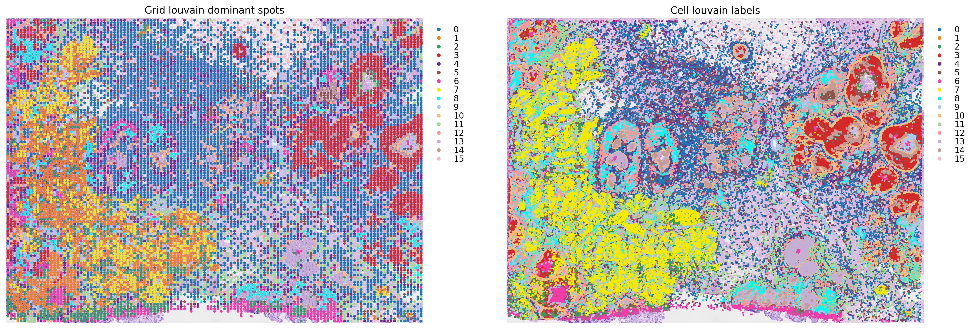
Checking the gridding
Comparing the gridded data to the original, to make sure it makes sense.
It’s recommend to visualise the dominant cell types per spot, in order to gauge whether the tissue structure is adequately maintained after gridding (i.e. to make sure it is not too low resolution!).
[14]:
fig, axes = plt.subplots(ncols=2, figsize=(20, 8))
st.pl.cluster_plot(grid, use_label='louvain', size=10, ax=axes[0], show_plot=False)
st.pl.cluster_plot(adata, use_label='louvain', ax=axes[1], show_plot=False)
axes[0].set_title(f'Grid louvain dominant spots')
axes[1].set_title(f'Cell louvain labels')
plt.show()
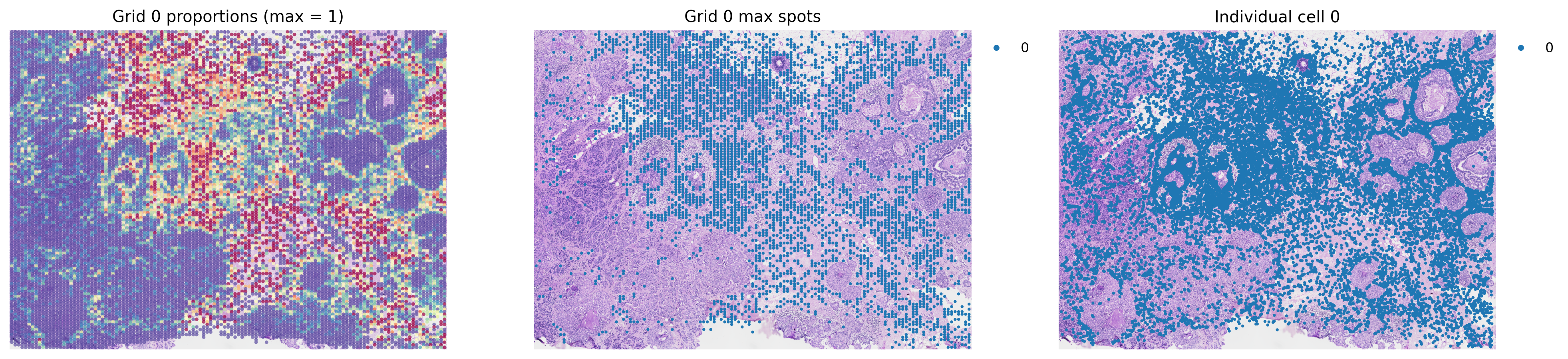
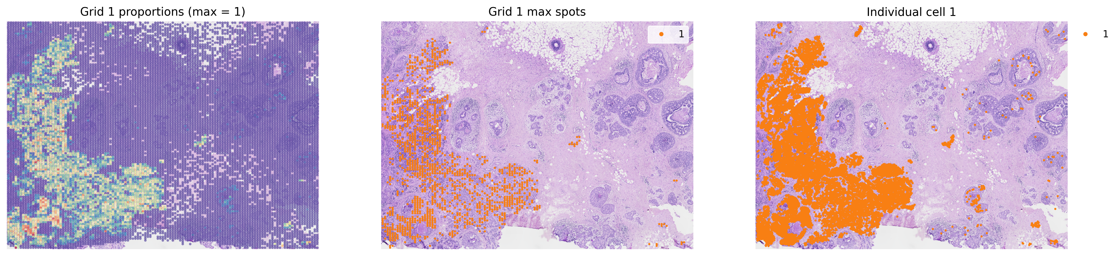
[15]:
groups = list(grid.obs['louvain'].cat.categories)
for group in groups[0:2]:
    fig, axes = plt.subplots(ncols=3, figsize=(20, 8))
    group_props = grid.uns['louvain'][group].values
    grid.obs['group'] = group_props
    st.pl.feat_plot(grid, feature='group', ax=axes[0], show_plot=False, vmax=1, show_color_bar=False)
    st.pl.cluster_plot(grid, use_label='louvain', list_clusters=[group], ax=axes[1], show_plot=False)
    st.pl.cluster_plot(adata, use_label='louvain', list_clusters=[group], ax=axes[2], show_plot=False)
    axes[0].set_title(f'Grid {group} proportions (max = 1)')
    axes[1].set_title(f'Grid {group} max spots')
    axes[2].set_title(f'Individual cell {group}')
    plt.show()
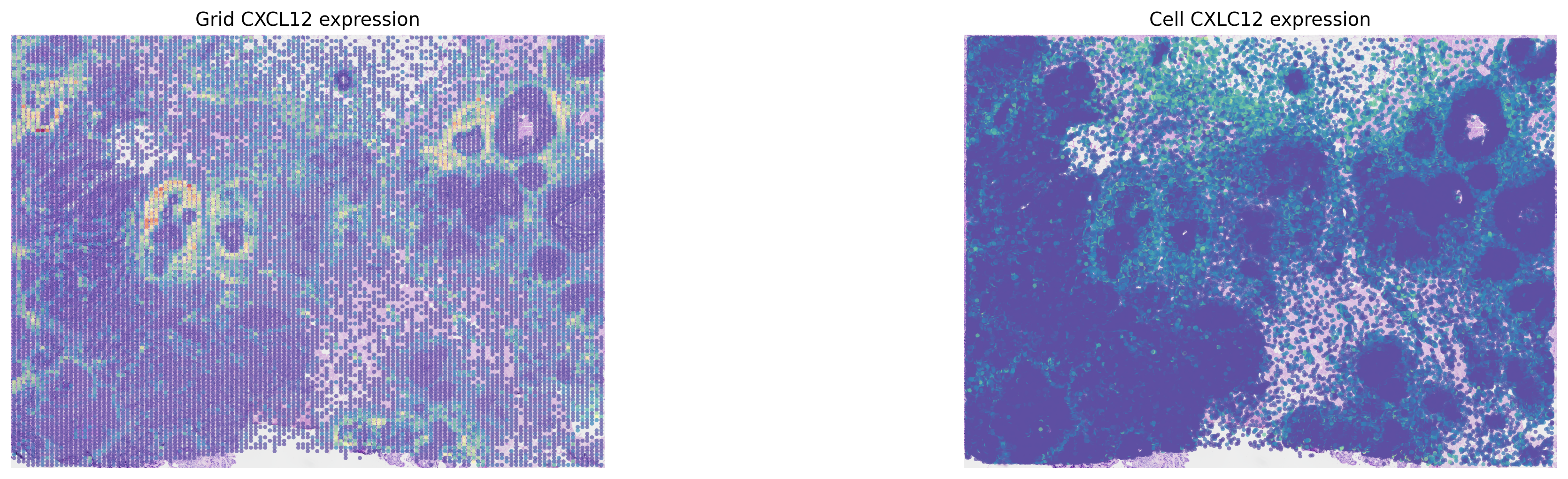
[16]:
fig, axes = plt.subplots(ncols=2, figsize=(20, 5))
st.pl.gene_plot(grid, gene_symbols='CXCL12', ax=axes[0], show_color_bar=False, show_plot=False)
st.pl.gene_plot(adata, gene_symbols='CXCL12', ax=axes[1], show_color_bar=False, show_plot=False, vmax=80)
axes[0].set_title(f'Grid CXCL12 expression')
axes[1].set_title(f'Cell CXLC12 expression')
plt.show()
LR Permutation Test
Running the LR permutation test, to determine regions of high LR co-expression.
[17]:
# Loading the LR databases available within stlearn (from NATMI)
lrs = st.tl.cci.load_lrs(['connectomeDB2020_lit'], species='human')
print(len(lrs))
2293
[18]:
# Running the analysis #
st.tl.cci.run(grid, lrs,
              min_spots=20,  # Filter out any LR pairs with no scores for less than min_spots
              distance=250,  # None defaults to spot+immediate neighbours; distance=0 for within-spot mode
              n_pairs=1000,  # Number of random pairs to generate; low as example, recommend ~10,000
              n_cpus=None,   # Number of CPUs for parallel. If None, detects & use all available.
              )
Calculating neighbours...
1 spots with no neighbours, 10 median spot neighbours.
Spot neighbour indices stored in adata.obsm['spot_neighbours'] & adata.obsm['spot_neigh_bcs'].
Altogether 20 valid L-R pairs
Generating backgrounds & testing each LR pair...: 100%|███████████████████████████████████████████████████████████████████████████████████████████████████████████████████████████████████████████████████████████████████████████████████████████████████████████████████████████████████████████████████ [ time left: 00:00 ]
Storing results:

lr_scores stored in adata.obsm['lr_scores'].
p_vals stored in adata.obsm['p_vals'].
p_adjs stored in adata.obsm['p_adjs'].
-log10(p_adjs) stored in adata.obsm['-log10(p_adjs)'].
lr_sig_scores stored in adata.obsm['lr_sig_scores'].

Per-spot results in adata.obsm have columns in same order as rows in adata.uns['lr_summary'].
Summary of LR results in adata.uns['lr_summary'].
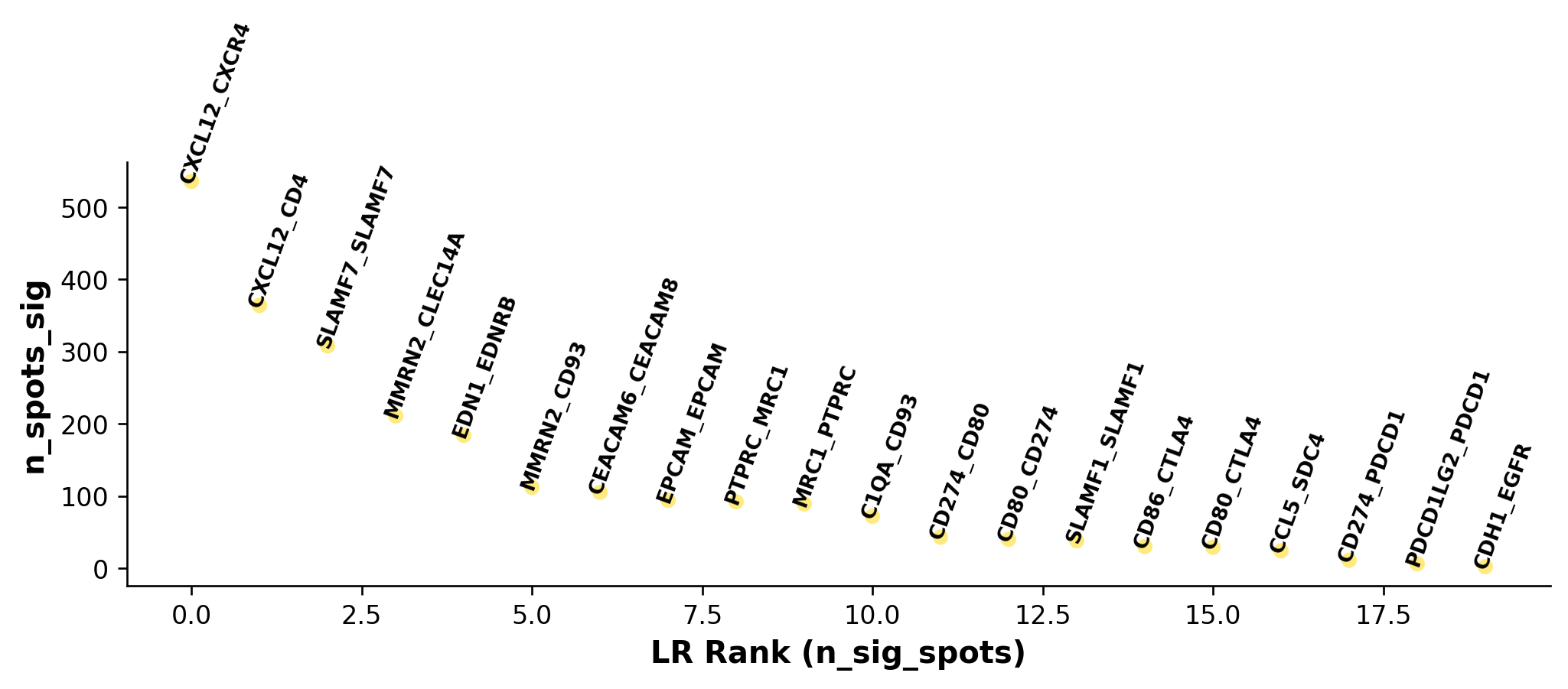
[19]:
lr_info = grid.uns['lr_summary']  # A dataframe detailing the LR pairs ranked by number of significant spots.
print(lr_info.shape)
print(lr_info)
(20, 3)
                 n_spots  n_spots_sig  n_spots_sig_pval
CXCL12_CXCR4       14215          536              2586
CXCL12_CD4         14057          364              3675
SLAMF7_SLAMF7       8162          308               789
MMRN2_CLEC14A       7961          211               821
EDN1_EDNRB          8249          184               882
MMRN2_CD93         10928          112               862
CEACAM6_CEACAM8    10562          105              1661
EPCAM_EPCAM        13271           94              2890
PTPRC_MRC1         13055           92              1088
MRC1_PTPRC         13055           89              1162
C1QA_CD93          12527           72               901
CD274_CD80          4944           43               281
CD80_CD274          4944           40               249
SLAMF1_SLAMF1       7660           38               344
CD86_CTLA4         10168           30               190
CD80_CTLA4          6094           29               226
CCL5_SDC4          12907           24               238
CD274_PDCD1         1756           11                65
PDCD1LG2_PDCD1      1902            6                63
CDH1_EGFR          13712            2               262
[20]:
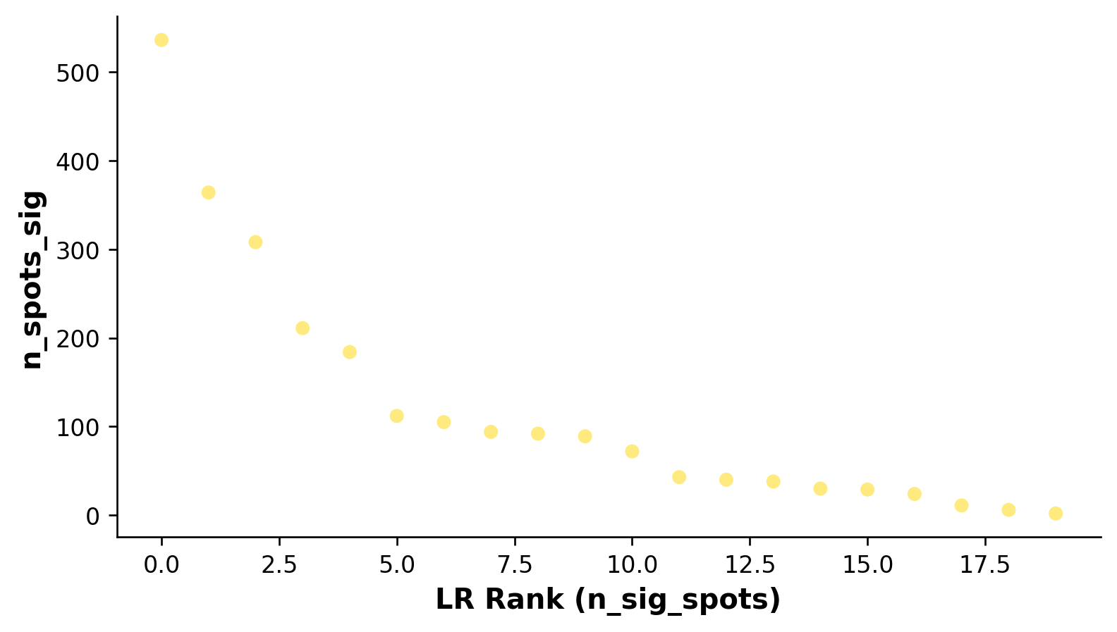
# Showing the rankings of the LR from a global and local perspective.
# Ranking based on number of significant hotspots.
st.pl.lr_summary(grid, n_top=500)
st.pl.lr_summary(grid, n_top=50, figsize=(10, 3))
Note: max_text (100) exceeds available LRs (20)
Note: max_text (100) exceeds available LRs (20)
[21]:
### Can adjust significance thresholds.
st.tl.cci.adj_pvals(grid, correct_axis='spot',
                    pval_adj_cutoff=0.05, adj_method='fdr_bh')
Updated adata.uns[lr_summary]
Updated adata.obsm[lr_scores]
Updated adata.obsm[lr_sig_scores]
Updated adata.obsm[p_vals]
Updated adata.obsm[p_adjs]
Updated adata.obsm[-log10(p_adjs)]
Downstream visualisations from LR analsyis
For more downstream visualisations, please see the stLearn CCI tutorial:
https://stlearn.readthedocs.io/en/latest/tutorials/stLearn-CCI.html
[22]:
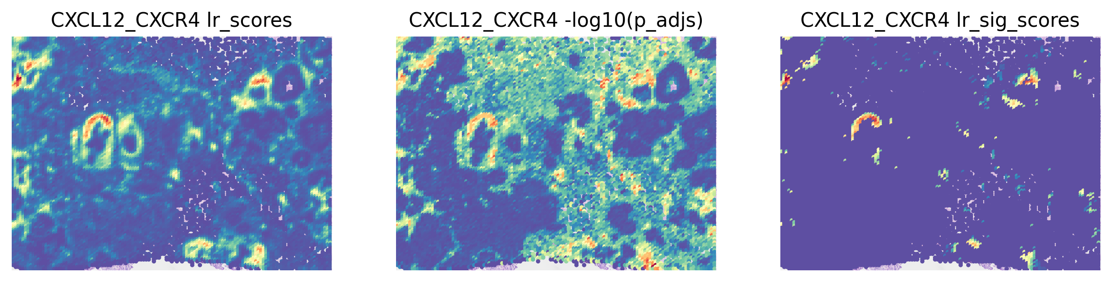
best_lr = grid.uns['lr_summary'].index.values[0] # Just choosing one of the top from lr_summary
[23]:
stats = ['lr_scores', '-log10(p_adjs)', 'lr_sig_scores']
fig, axes = plt.subplots(ncols=len(stats), figsize=(12, 6))
for i, stat in enumerate(stats):
    st.pl.lr_result_plot(grid, use_result=stat, use_lr=best_lr, show_color_bar=False, ax=axes[i])
    axes[i].set_title(f'{best_lr} {stat}')
Predicting Significant Cell-Cell Interactions
For this analysis, we are using within-spot mode, with the deconvolution information which is stored in grid.uns, as automatically determined by st.tl.cci.grid. The permutation is performed to permute the cell proportions associated with each spot, to determine spots located in LR hotspots that have certain cell types over-represented.
[24]:
grid
[24]:
AnnData object with n_obs × n_vars = 14364 × 313
    obs: 'imagecol', 'imagerow', 'n_cells', 'louvain', 'group'
    uns: 'spatial', 'louvain', 'louvain_colors', 'grid_counts', 'grid_xedges', 'grid_yedges', 'lrfeatures', 'lr_summary'
    obsm: 'spatial', 'spot_neighbours', 'spot_neigh_bcs', 'lr_scores', 'p_vals', 'p_adjs', '-log10(p_adjs)', 'lr_sig_scores'
[25]:
st.tl.cci.run_cci(grid, 'louvain',  # Spot cell information either in data.obs or data.uns
                  min_spots=2,  # Minimum number of spots for LR to be tested.
                  spot_mixtures=True,  # If True will use the deconvolution data,
                  # so spots can have multiple cell types if score>cell_prop_cutoff
                  cell_prop_cutoff=0.1,  # Spot considered to have cell type if score>0.1
                  sig_spots=True,  # Only consider neighbourhoods of spots which had significant LR scores.
                  n_perms=100,  # Permutations of cell information to get background, recommend ~1000
                  n_cpus=None,
                  )
Getting cached neighbourhood information...
Getting information for CCI counting...
Counting celltype-celltype interactions per LR and permuting 100 times.: 100%|████████████████████████████████████████████████████████████████████████████████████████████████████████████████████████████████████████████████████████████████████████████████████████████████████████████████████████████ [ time left: 00:00 ]
Significant counts of cci_rank interactions for all LR pairs in data.uns[lr_cci_louvain]
Significant counts of cci_rank interactions for each LR pair stored in dictionary data.uns[per_lr_cci_louvain]
[26]:
st.tl.cci.run_cci(grid, 'louvain',  # Spot cell information either in data.obs or data.uns
                  min_spots=2,  # Minimum number of spots for LR to be tested.
                  spot_mixtures=True,  # If True will use the deconvolution data,
                  # so spots can have multiple cell types if score>cell_prop_cutoff
                  cell_prop_cutoff=0.1,  # Spot considered to have cell type if score>0.1
                  sig_spots=True,  # Only consider neighbourhoods of spots which had significant LR scores.
                  n_perms=100,  # Permutations of cell information to get background, recommend ~1000
                  n_cpus=10,
                  )
Getting cached neighbourhood information...
Getting information for CCI counting...
Counting celltype-celltype interactions per LR and permuting 100 times.: 100%|████████████████████████████████████████████████████████████████████████████████████████████████████████████████████████████████████████████████████████████████████████████████████████████████████████████████████████████ [ time left: 00:00 ]
Significant counts of cci_rank interactions for all LR pairs in data.uns[lr_cci_louvain]
Significant counts of cci_rank interactions for each LR pair stored in dictionary data.uns[per_lr_cci_louvain]
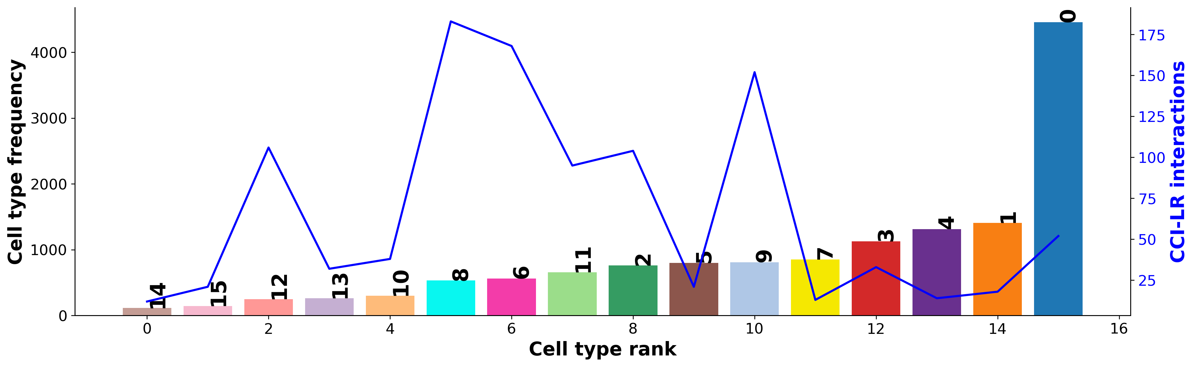
Diagnostic: checking for interaction and cell type frequency correlation
Should be little to no correlation; indicating the permutation has adequately controlled for cell type frequency.
[27]:
st.pl.cci_check(grid, 'louvain', figsize=(16, 5))
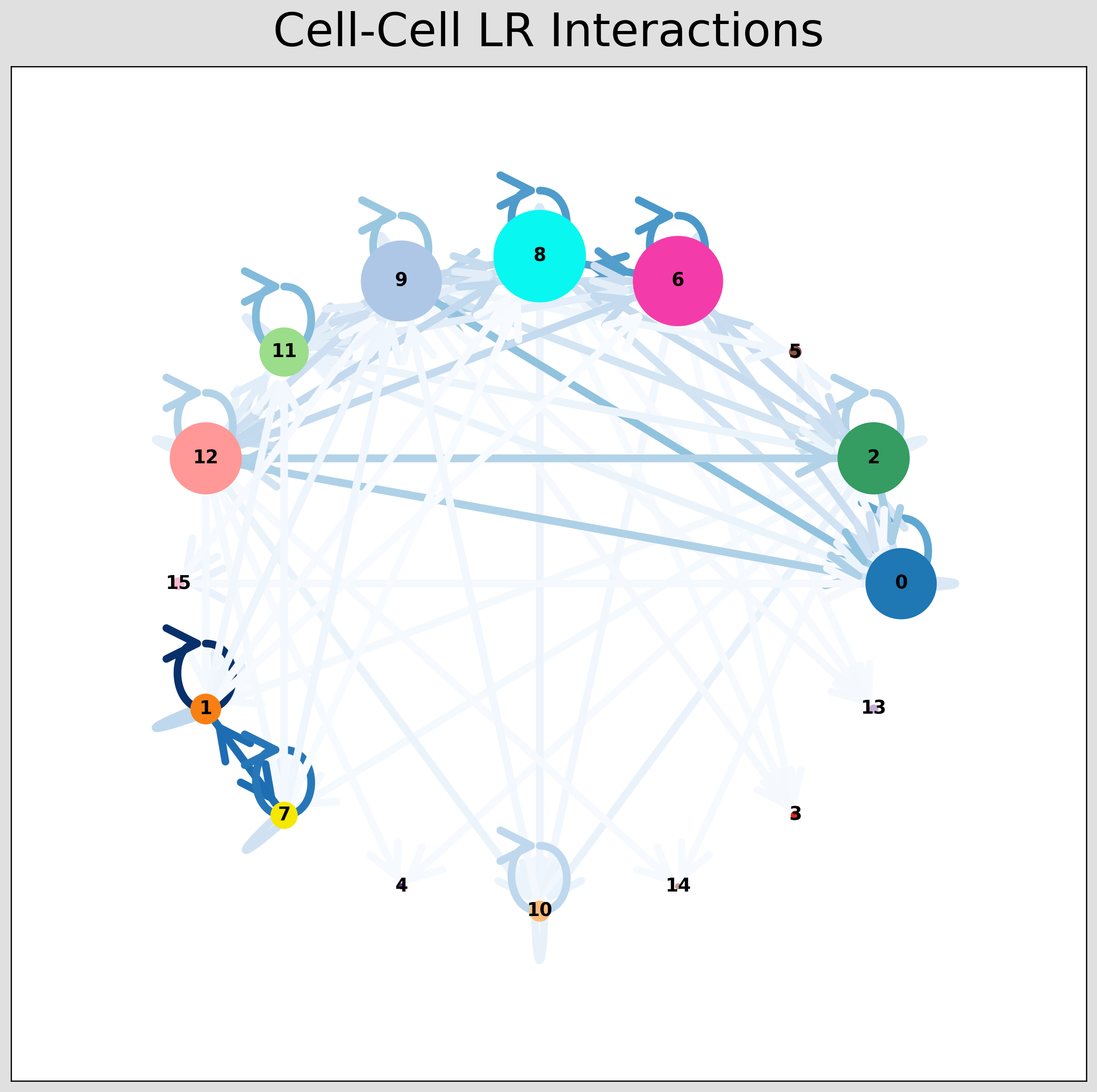
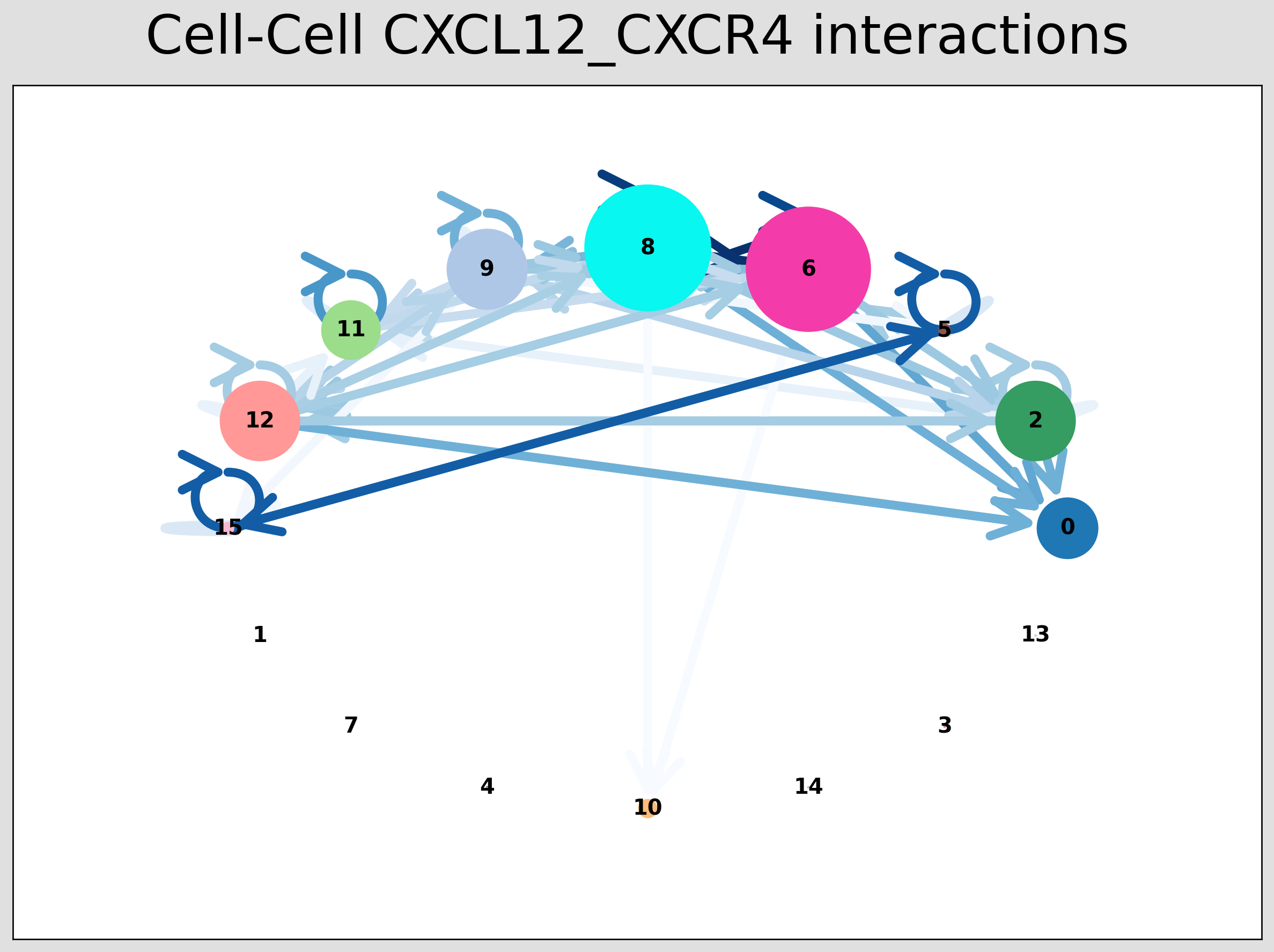
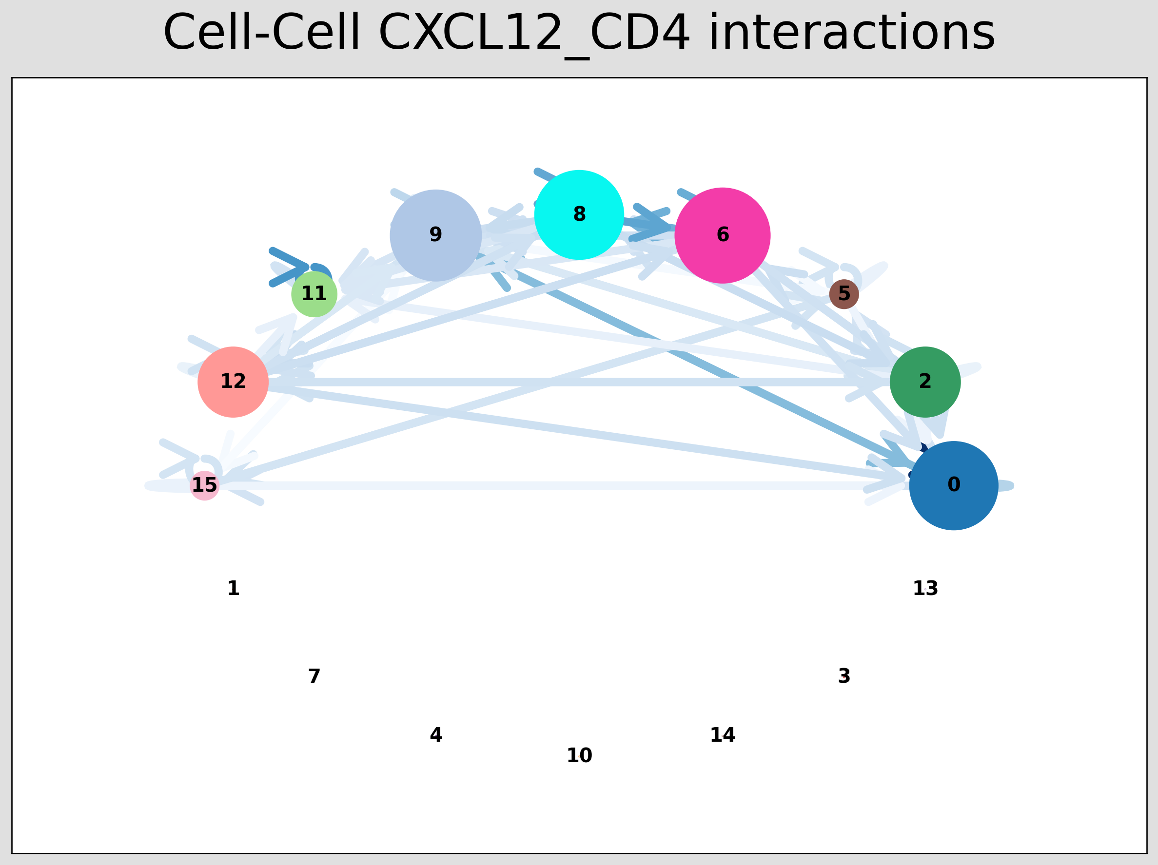
CCI Visualisations
CCI Network Plot
[28]:
# Visualising the no. of interactions between cell types across all LR pairs #
pos_1 = st.pl.ccinet_plot(grid, 'louvain', return_pos=True, min_counts=30)

# Just examining the cell type interactions between selected pairs #
lrs = grid.uns['lr_summary'].index.values[0:3]
for best_lr in lrs[0:2]:
    st.pl.ccinet_plot(grid, 'louvain', best_lr, min_counts=2,
                      figsize=(10, 7.5), pos=pos_1,
                      )
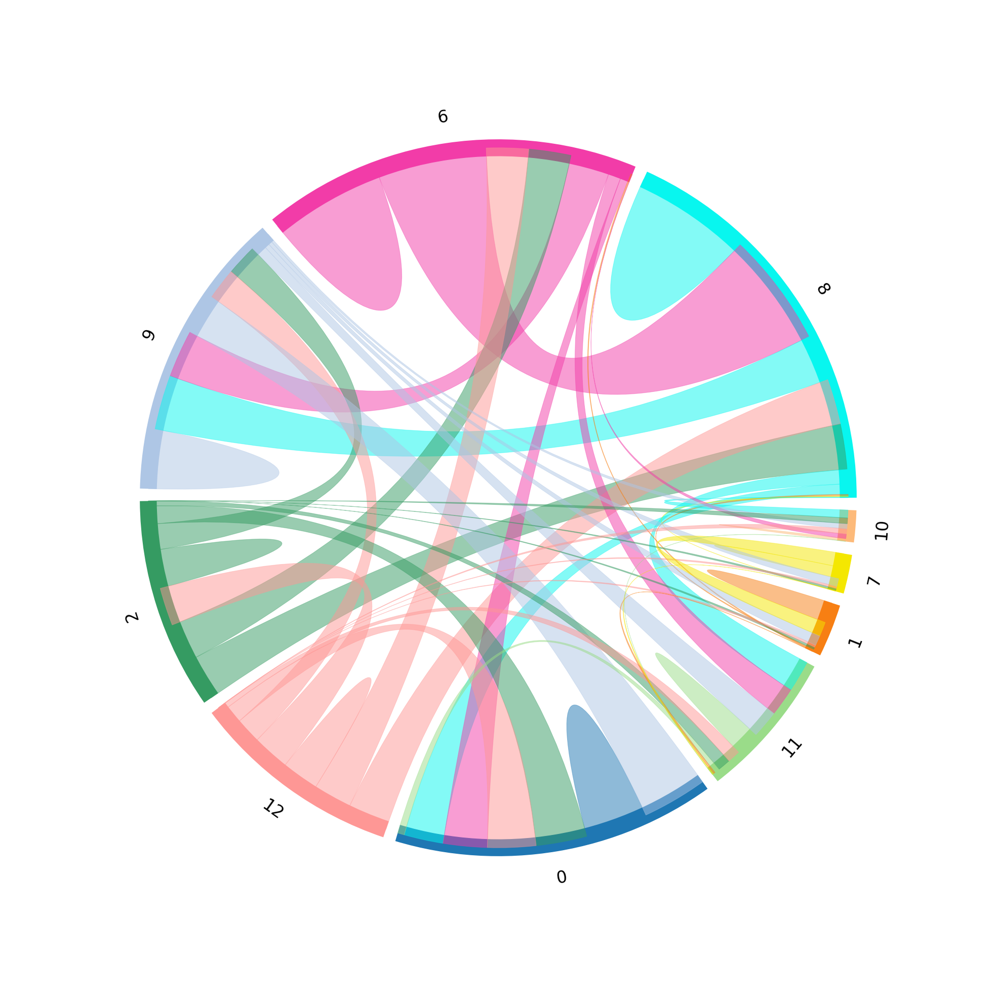
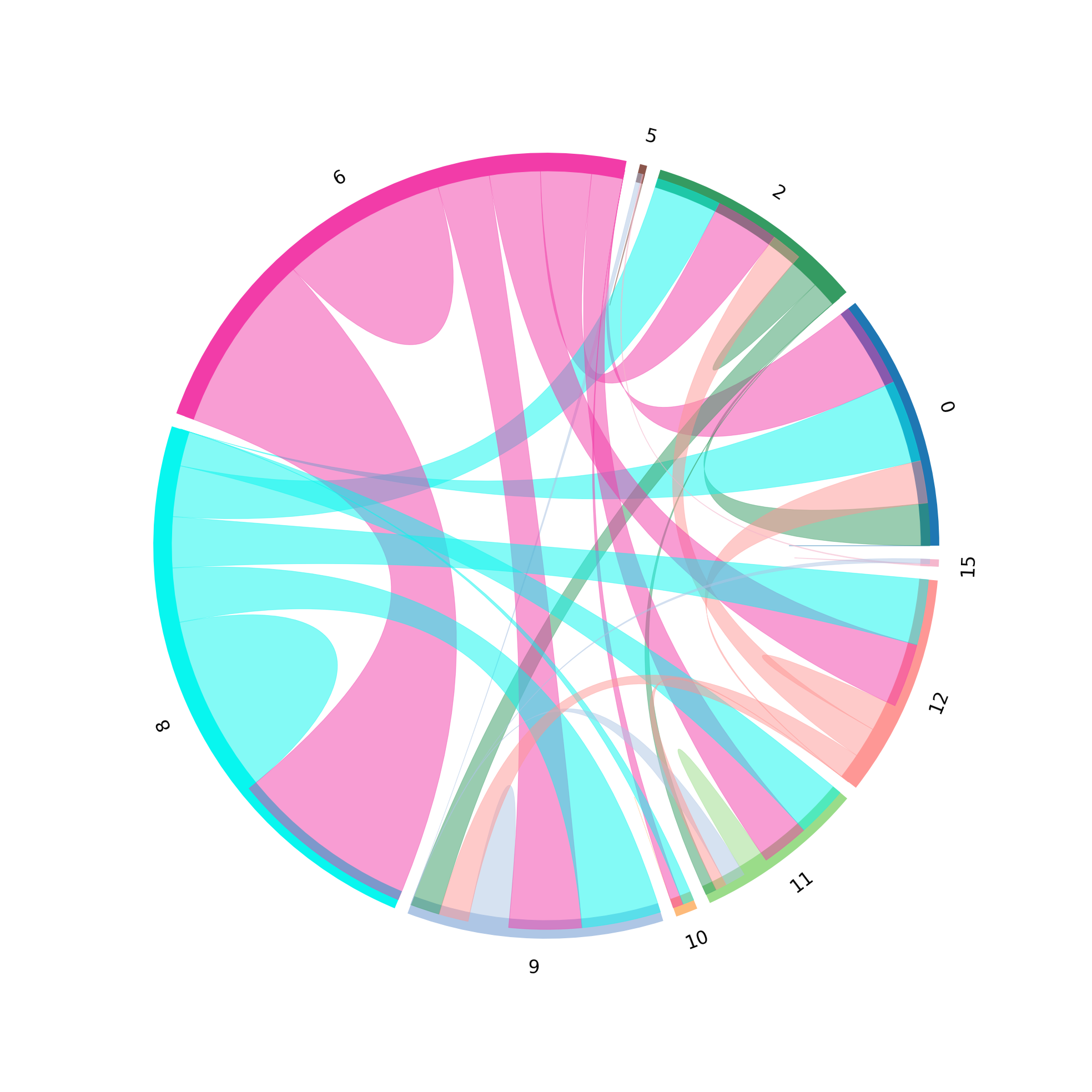
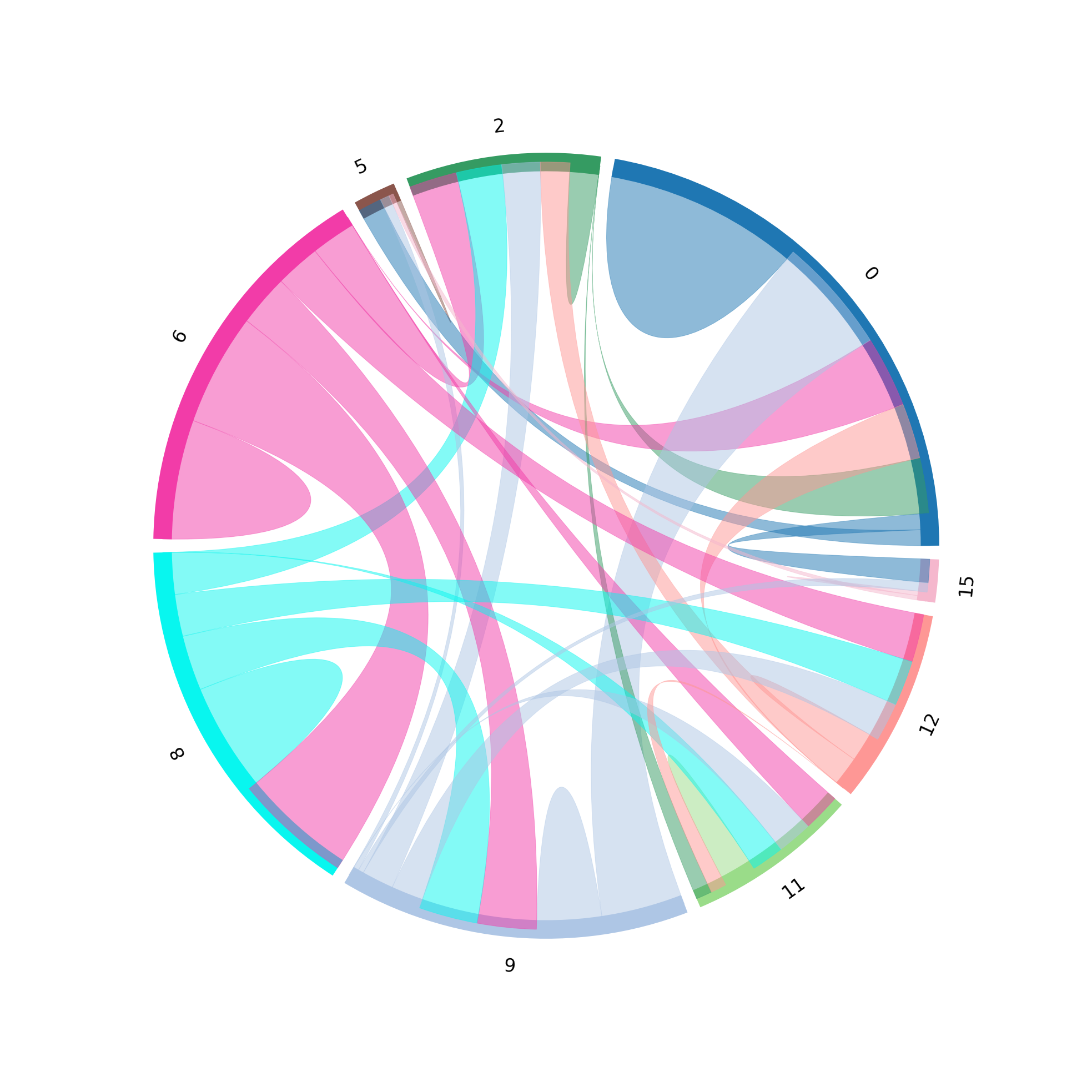
CCI Chord Plot
[29]:
st.pl.lr_chord_plot(grid, 'louvain')

for lr in lrs[0:2]:
    st.pl.lr_chord_plot(grid, 'louvain', lr)
For additional visualisations and visualisation tips, please see:
https://stlearn.readthedocs.io/en/latest/tutorials/stLearn-CCI.html
Acknowledgement
We would like to thank Soo Hee Lee and 10X Genomics team for their able support, contribution and feedback to this tutorial