Pseudotime Spatial Trajectory Inference¶

In this tutorial, we are using both spatial information and gene expression profile to perform spatial trajectory inference to explore the progression of Ductal Carcinoma in situ (DCIS) - Invasive Ductal Cancer (IDC)

Source: https://www.10xgenomics.com/datasets/human-breast-cancer-block-a-section-1-1-standard-1-1-0

1. Preparation¶

We are trying to keep it focus on spatial trajectory inference then every step from reading data, processing to clustering, we will give the code here to easier for user to use.

Read and preprocess data¶

[1]:

import stlearn as st
import pathlib as pathlib

st.settings.set_figure_params(dpi=120)

# Ignore all warnings
import warnings
warnings.filterwarnings("ignore")

/Users/andrew/conda/stlearn/lib/python3.10/site-packages/louvain/__init__.py:54: UserWarning: pkg_resources is deprecated as an API. See https://setuptools.pypa.io/en/latest/pkg_resources.html. The pkg_resources package is slated for removal as early as 2025-11-30. Refrain from using this package or pin to Setuptools<81.
  from pkg_resources import get_distribution, DistributionNotFound
/Users/andrew/conda/stlearn/lib/python3.10/site-packages/stlearn/tl/cci/het.py:206: NumbaDeprecationWarning: The keyword argument 'nopython=False' was supplied. From Numba 0.59.0 the default is being changed to True and use of 'nopython=False' will raise a warning as the argument will have no effect. See https://numba.readthedocs.io/en/stable/reference/deprecation.html#deprecation-of-object-mode-fall-back-behaviour-when-using-jit for details.
  @jit(parallel=True, nopython=False)

[2]:

# Read raw data
st.settings.datasetdir = pathlib.Path.cwd().parent / "data"
data = st.datasets.visium_sge(sample_id="V1_Breast_Cancer_Block_A_Section_1")
data = st.convert_scanpy(data)

[3]:

# Save raw_count
data.layers["raw_count"] = data.X
# Preprocessing
st.pp.filter_genes(data, min_cells=3)
st.pp.normalize_total(data)
st.pp.log1p(data)
# Keep raw data
data.raw = data
st.pp.scale(data)

Normalization step is finished in adata.X
Log transformation step is finished in adata.X
Scale step is finished in adata.X

Clustering data¶

[4]:

# Run PCA
st.em.run_pca(data, n_comps=50, random_state=0)
# Tiling image
st.pp.tiling(data, out_path="tiling", crop_size=40)
# Using Deep Learning to extract feature
st.pp.extract_feature(data)
# Apply stSME spatial-PCA option
st.spatial.morphology.adjust(data, use_data="X_pca", radius=50, method="mean")
st.pp.neighbors(data, n_neighbors=25, use_rep='X_pca_morphology', random_state=0)
st.tl.clustering.louvain(data, random_state=0)

PCA is done! Generated in adata.obsm['X_pca'], adata.uns['pca'] and adata.varm['PCs']

Tiling image: 100%|███████████████████████████████████████████████████████████████████████████████████████████████████████████████████████████████████████████████████████████████████████████████████████████████████████████████████████████████████████████████████████████████████████████████████████ [ time left: 00:00 ]
Extract feature:  97%|████████████████████████████████████████████████████████████████████████████████████████████████████████████████████████████████████████████████████████████████████████████████████████████████████████████████████████████████████████████████████████████████████████████▉        [ time left: 00:07 ]

The morphology feature is added to adata.obsm['X_morphology']!

Adjusting data: 100%|█████████████████████████████████████████████████████████████████████████████████████████████████████████████████████████████████████████████████████████████████████████████████████████████████████████████████████████████████████████████████████████████████████████████████████ [ time left: 00:00 ]

The data adjusted by morphology is added to adata.obsm['X_pca_morphology']

OMP: Info #276: omp_set_nested routine deprecated, please use omp_set_max_active_levels instead.

Created k-Nearest-Neighbor graph in adata.uns['neighbors']
Applying Louvain cluster ...
Louvain cluster is done! The labels are stored in adata.obs['louvain']

[5]:

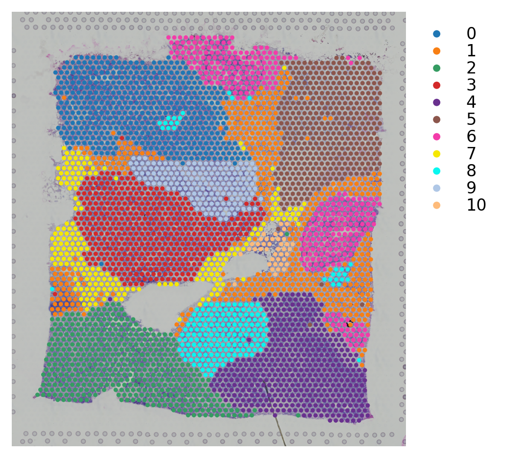
st.pl.cluster_plot(data, use_label="louvain", image_alpha=1, size=7)

[5]:

AnnData object with n_obs × n_vars = 3798 × 22240
    obs: 'in_tissue', 'array_row', 'array_col', 'imagecol', 'imagerow', 'tile_path', 'louvain'
    var: 'gene_ids', 'feature_types', 'genome', 'n_cells', 'mean', 'std'
    uns: 'spatial', 'log1p', 'pca', 'neighbors', 'louvain', 'louvain_colors'
    obsm: 'spatial', 'X_pca', 'X_tile_feature', 'X_morphology', 'X_pca_morphology'
    varm: 'PCs'
    layers: 'raw_count'
    obsp: 'distances', 'connectivities'

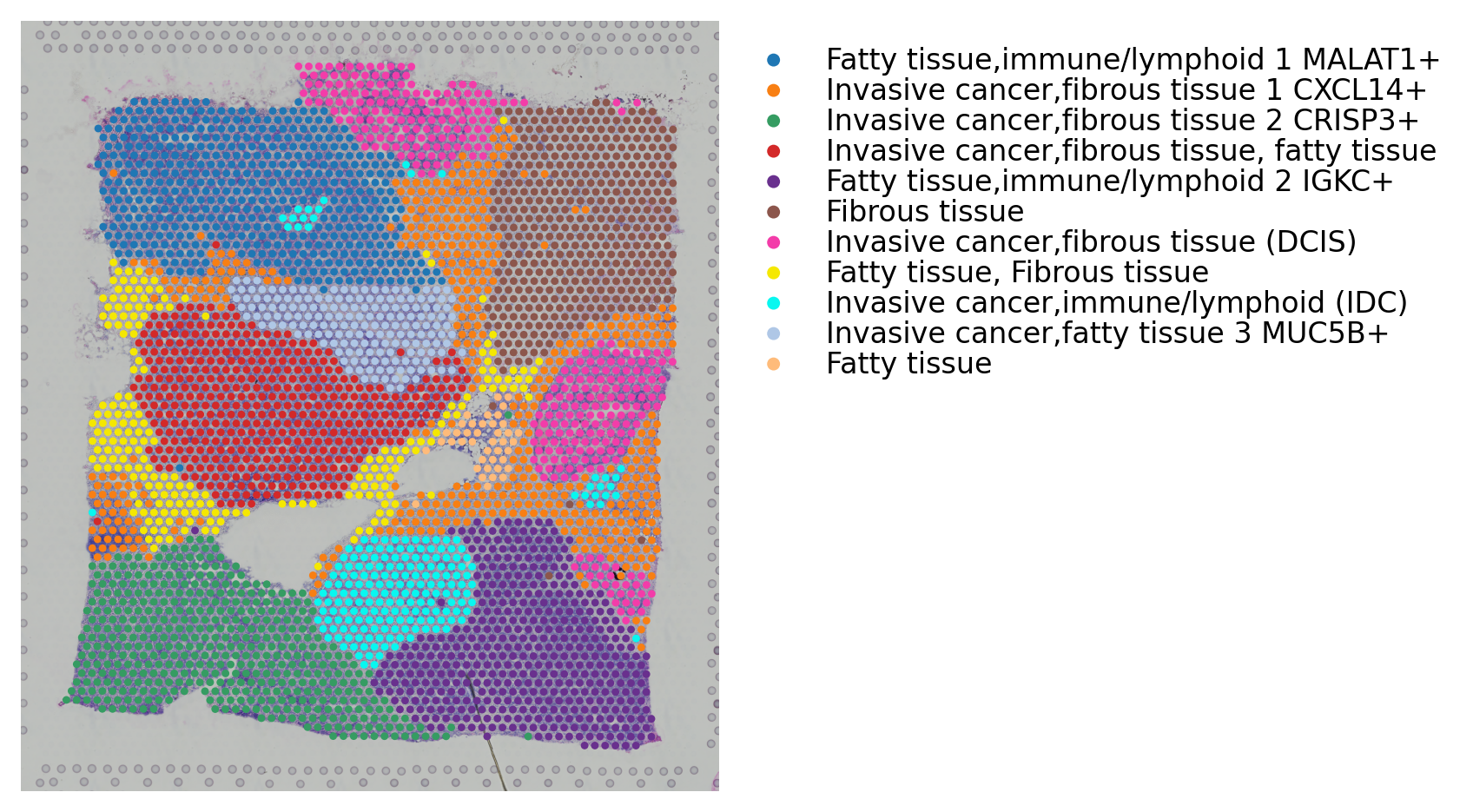
../_images/tutorials_pseudotime_space_10_1.png

[6]:

st.add.annotation(data, label_list=['Fatty tissue,immune/lymphoid 1 MALAT1+',
                                    'Invasive cancer,fibrous tissue 1 CXCL14+',
                                    'Invasive cancer,fibrous tissue 2 CRISP3+',
                                    'Invasive cancer,fibrous tissue, fatty tissue',
                                    'Fatty tissue,immune/lymphoid 2 IGKC+',
                                    'Fibrous tissue',
                                    'Invasive cancer,fibrous tissue (DCIS)',
                                    'Fatty tissue, Fibrous tissue',
                                    'Invasive cancer,immune/lymphoid (IDC)',
                                    'Invasive cancer,fatty tissue 3 MUC5B+',
                                    'Fatty tissue'],
                  use_label="louvain")
st.pl.cluster_plot(data, use_label="louvain_anno", image_alpha=1, size=7)

The annotation is added to adata.obs['louvain_anno']

[6]:

AnnData object with n_obs × n_vars = 3798 × 22240
    obs: 'in_tissue', 'array_row', 'array_col', 'imagecol', 'imagerow', 'tile_path', 'louvain', 'louvain_anno'
    var: 'gene_ids', 'feature_types', 'genome', 'n_cells', 'mean', 'std'
    uns: 'spatial', 'log1p', 'pca', 'neighbors', 'louvain', 'louvain_colors', 'louvain_anno_colors'
    obsm: 'spatial', 'X_pca', 'X_tile_feature', 'X_morphology', 'X_pca_morphology'
    varm: 'PCs'
    layers: 'raw_count'
    obsp: 'distances', 'connectivities'

../_images/tutorials_pseudotime_space_11_2.png

2. Spatial trajectory inference¶

Choosing root¶

3733 is the index of the spot that we chose as root. It in the DCIS cluster (6). We recommend the root spot should be in the end/begin of a cluster in UMAP space. You can find min/max point of a cluster in UMAP as root.

[7]:

data.uns["iroot"] = st.spatial.trajectory.set_root(data, use_label="louvain", cluster="6", use_raw=True)
st.spatial.trajectory.pseudotime(data, eps=50, use_rep="X_pca", use_label="louvain")

All available trajectory paths are stored in adata.uns['available_paths'] with length < 4 nodes

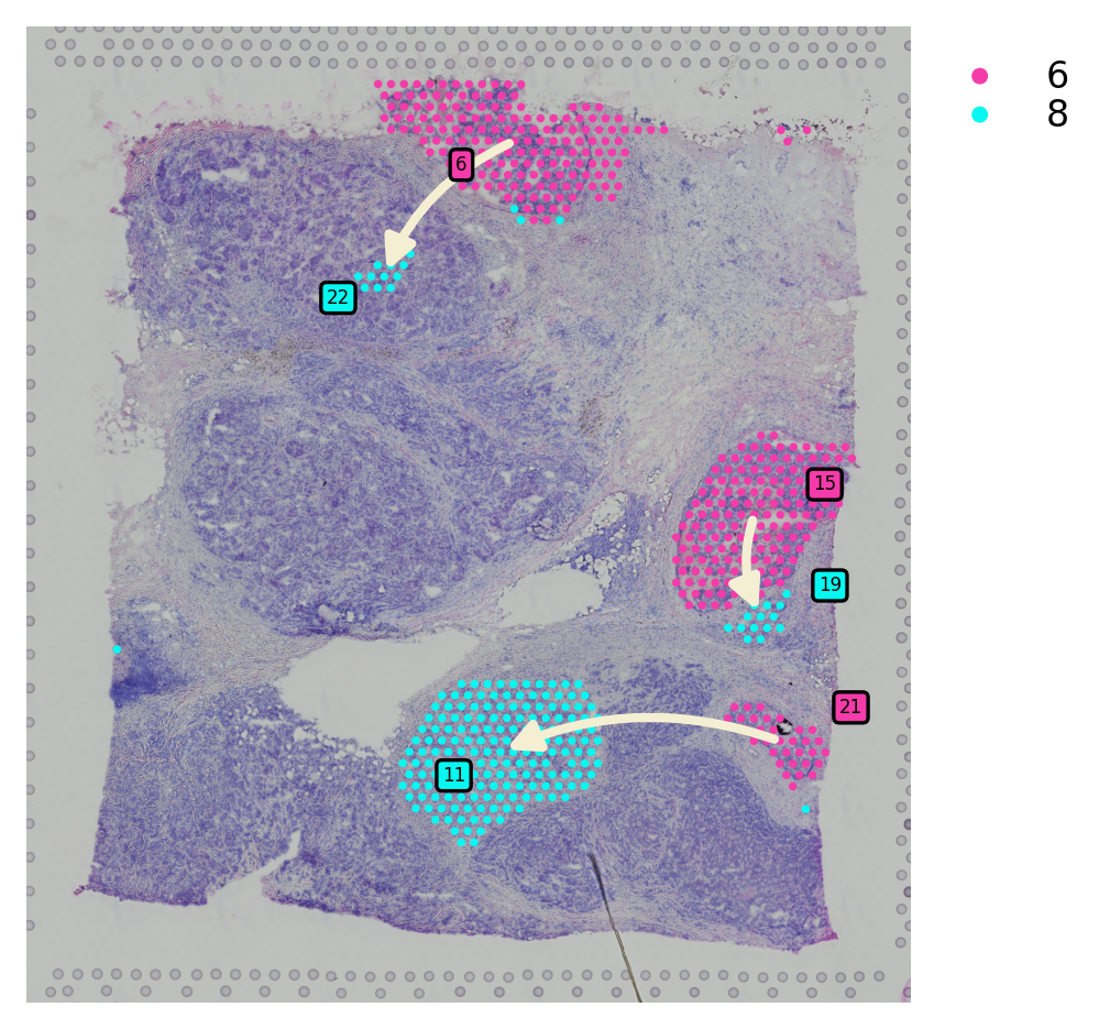
Spatial trajectory inference - global level¶

We run the global level of pseudo-time-space (PSTS) method to reconstruct the spatial trajectory between cluster 6 (DCIS) and 8 (lesions IDC)

[8]:

st.spatial.trajectory.pseudotimespace_global(data, use_label="louvain", list_clusters=["6", "8"])

Start to construct the trajectory: 6 -> 8

[8]:

AnnData object with n_obs × n_vars = 3798 × 22240
    obs: 'in_tissue', 'array_row', 'array_col', 'imagecol', 'imagerow', 'tile_path', 'louvain', 'louvain_anno', 'sub_cluster_labels', 'dpt_pseudotime'
    var: 'gene_ids', 'feature_types', 'genome', 'n_cells', 'mean', 'std'
    uns: 'spatial', 'log1p', 'pca', 'neighbors', 'louvain', 'louvain_colors', 'louvain_anno_colors', 'iroot', 'louvain_index_dict', 'paga', 'louvain_sizes', 'diffmap_evals', 'threshold_spots', 'split_node', 'global_graph', 'centroid_dict', 'available_paths', 'PTS_graph'
    obsm: 'spatial', 'X_pca', 'X_tile_feature', 'X_morphology', 'X_pca_morphology', 'X_diffmap'
    varm: 'PCs'
    layers: 'raw_count'
    obsp: 'distances', 'connectivities'

[9]:

st.pl.cluster_plot(data, use_label="louvain", show_trajectories=True, list_clusters=["6", "8"], show_subcluster=True)

[9]:

AnnData object with n_obs × n_vars = 3798 × 22240
    obs: 'in_tissue', 'array_row', 'array_col', 'imagecol', 'imagerow', 'tile_path', 'louvain', 'louvain_anno', 'sub_cluster_labels', 'dpt_pseudotime'
    var: 'gene_ids', 'feature_types', 'genome', 'n_cells', 'mean', 'std'
    uns: 'spatial', 'log1p', 'pca', 'neighbors', 'louvain', 'louvain_colors', 'louvain_anno_colors', 'iroot', 'louvain_index_dict', 'paga', 'louvain_sizes', 'diffmap_evals', 'threshold_spots', 'split_node', 'global_graph', 'centroid_dict', 'available_paths', 'PTS_graph'
    obsm: 'spatial', 'X_pca', 'X_tile_feature', 'X_morphology', 'X_pca_morphology', 'X_diffmap'
    varm: 'PCs'
    layers: 'raw_count'
    obsp: 'distances', 'connectivities'

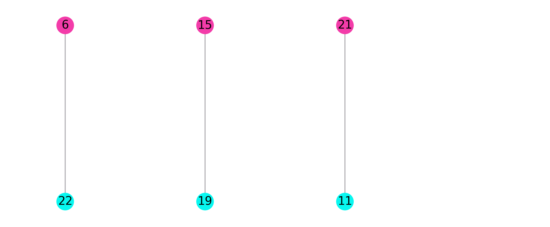
../_images/tutorials_pseudotime_space_17_1.png

[10]:

st.pl.trajectory.tree_plot(data)

../_images/tutorials_pseudotime_space_18_0.png

[10]:

AnnData object with n_obs × n_vars = 3798 × 22240
    obs: 'in_tissue', 'array_row', 'array_col', 'imagecol', 'imagerow', 'tile_path', 'louvain', 'louvain_anno', 'sub_cluster_labels', 'dpt_pseudotime'
    var: 'gene_ids', 'feature_types', 'genome', 'n_cells', 'mean', 'std'
    uns: 'spatial', 'log1p', 'pca', 'neighbors', 'louvain', 'louvain_colors', 'louvain_anno_colors', 'iroot', 'louvain_index_dict', 'paga', 'louvain_sizes', 'diffmap_evals', 'threshold_spots', 'split_node', 'global_graph', 'centroid_dict', 'available_paths', 'PTS_graph'
    obsm: 'spatial', 'X_pca', 'X_tile_feature', 'X_morphology', 'X_pca_morphology', 'X_diffmap'
    varm: 'PCs'
    layers: 'raw_count'
    obsp: 'distances', 'connectivities'

Transition markers detection¶

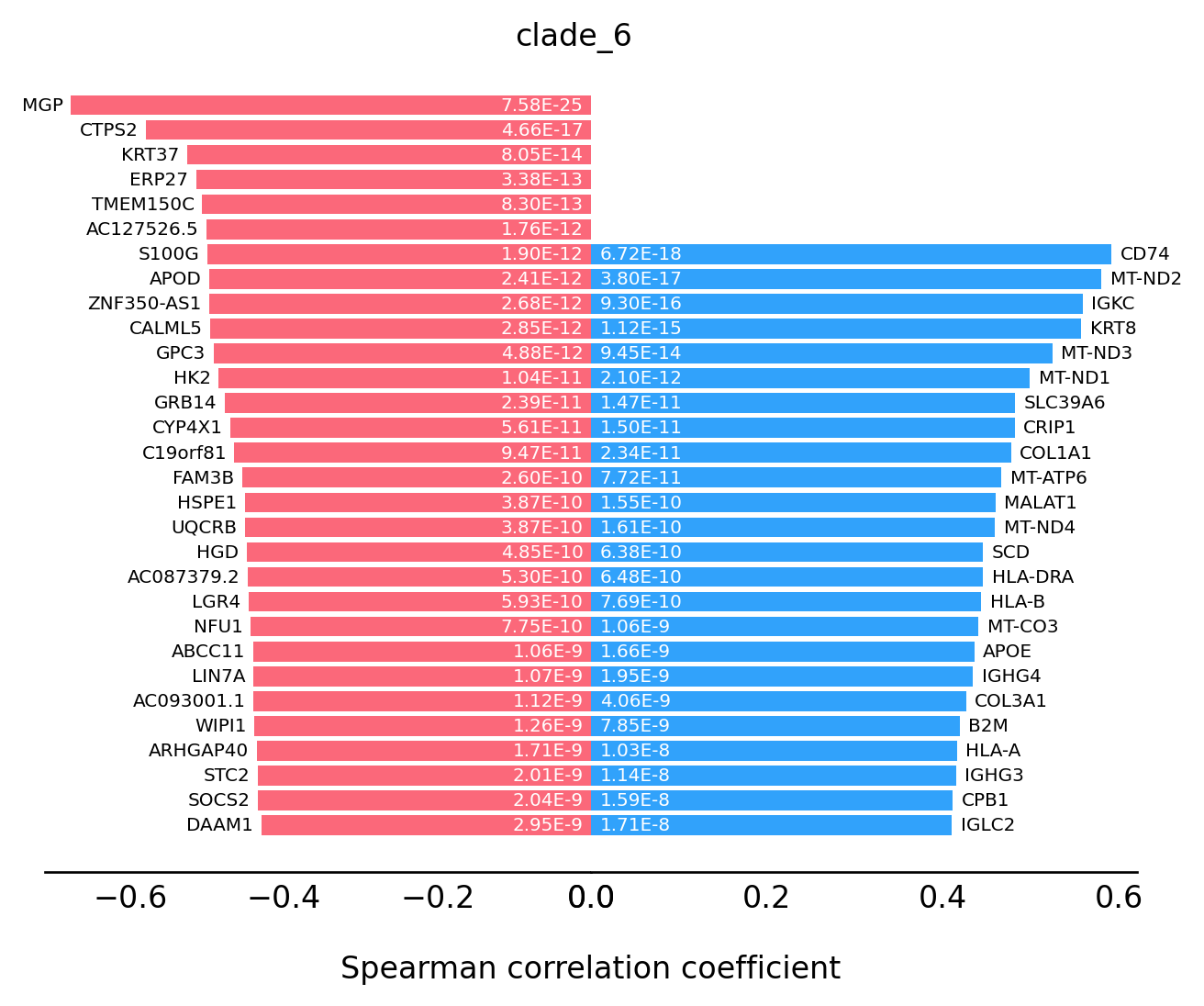
Based on the spatial trajectory/tree plot, we can see 2 clades are started from sub-cluster 6 and 15. Then we run the function to detect the highly correlated genes with the PSTS values.

[11]:

st.spatial.trajectory.detect_transition_markers_clades(data, clade=6, use_raw_count=False, cutoff_spearman=0.4)

Detecting the transition markers of clade_6...
Transition markers result is stored in adata.uns['clade_6']

[12]:

st.spatial.trajectory.detect_transition_markers_clades(data, clade=15, use_raw_count=False, cutoff_spearman=0.4)

Detecting the transition markers of clade_15...
Transition markers result is stored in adata.uns['clade_15']

[13]:

st.spatial.trajectory.detect_transition_markers_clades(data, clade=21, use_raw_count=False, cutoff_spearman=0.4)

Detecting the transition markers of clade_21...
Transition markers result is stored in adata.uns['clade_21']

[14]:

data.uns['clade_6'] = data.uns['clade_6'][data.uns['clade_6']['gene'].map(lambda x: "RPL" not in x)]
data.uns['clade_15'] = data.uns['clade_15'][data.uns['clade_15']['gene'].map(lambda x: "RPL" not in x)]
data.uns['clade_21'] = data.uns['clade_21'][data.uns['clade_21']['gene'].map(lambda x: "RPL" not in x)]
data.uns['clade_6'] = data.uns['clade_6'][data.uns['clade_6']['gene'].map(lambda x: "RPS" not in x)]
data.uns['clade_15'] = data.uns['clade_15'][data.uns['clade_15']['gene'].map(lambda x: "RPS" not in x)]
data.uns['clade_21'] = data.uns['clade_21'][data.uns['clade_21']['gene'].map(lambda x: "RPS" not in x)]

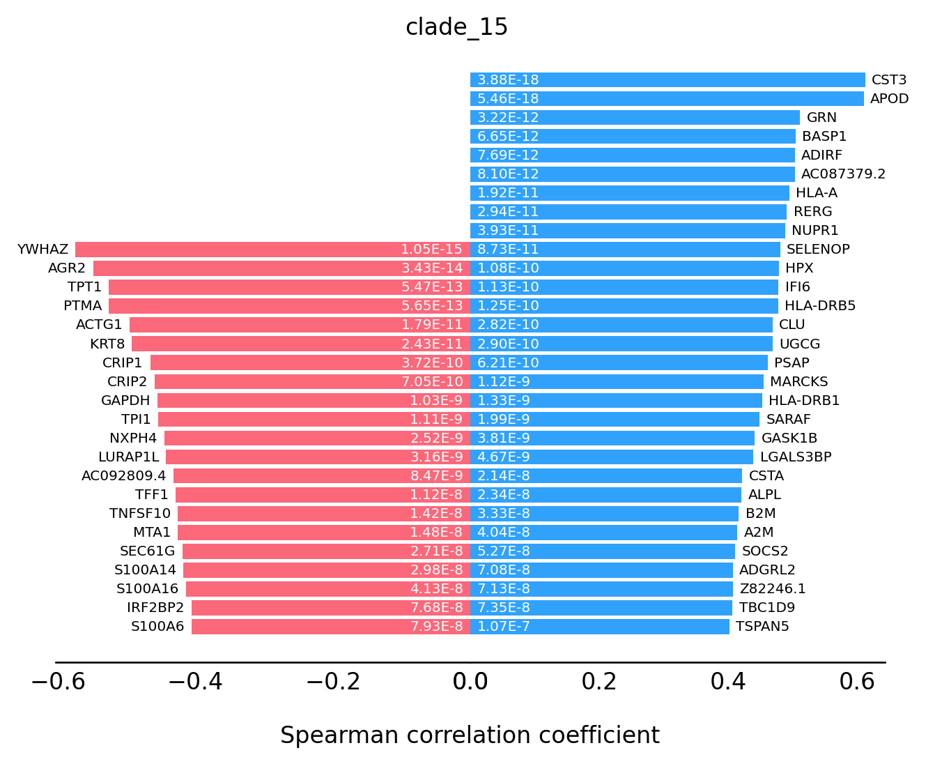
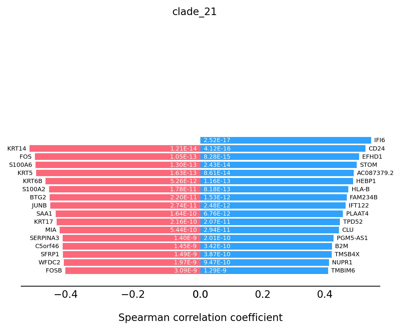
For the transition markers plot, genes from left side (red) are negatively correlated with the spatial trajectory and genes from right side (blue) are positively correlated with the spatial trajectory.

[15]:

st.pl.trajectory.transition_markers_plot(data, top_genes=30, trajectory="clade_6")

../_images/tutorials_pseudotime_space_25_0.png

[15]:

AnnData object with n_obs × n_vars = 3798 × 22240
    obs: 'in_tissue', 'array_row', 'array_col', 'imagecol', 'imagerow', 'tile_path', 'louvain', 'louvain_anno', 'sub_cluster_labels', 'dpt_pseudotime'
    var: 'gene_ids', 'feature_types', 'genome', 'n_cells', 'mean', 'std'
    uns: 'spatial', 'log1p', 'pca', 'neighbors', 'louvain', 'louvain_colors', 'louvain_anno_colors', 'iroot', 'louvain_index_dict', 'paga', 'louvain_sizes', 'diffmap_evals', 'threshold_spots', 'split_node', 'global_graph', 'centroid_dict', 'available_paths', 'PTS_graph', 'clade_6', 'clade_15', 'clade_21'
    obsm: 'spatial', 'X_pca', 'X_tile_feature', 'X_morphology', 'X_pca_morphology', 'X_diffmap'
    varm: 'PCs'
    layers: 'raw_count'
    obsp: 'distances', 'connectivities'

[16]:

st.pl.trajectory.transition_markers_plot(data, top_genes=30, trajectory="clade_15")

../_images/tutorials_pseudotime_space_26_0.png

[16]:

AnnData object with n_obs × n_vars = 3798 × 22240
    obs: 'in_tissue', 'array_row', 'array_col', 'imagecol', 'imagerow', 'tile_path', 'louvain', 'louvain_anno', 'sub_cluster_labels', 'dpt_pseudotime'
    var: 'gene_ids', 'feature_types', 'genome', 'n_cells', 'mean', 'std'
    uns: 'spatial', 'log1p', 'pca', 'neighbors', 'louvain', 'louvain_colors', 'louvain_anno_colors', 'iroot', 'louvain_index_dict', 'paga', 'louvain_sizes', 'diffmap_evals', 'threshold_spots', 'split_node', 'global_graph', 'centroid_dict', 'available_paths', 'PTS_graph', 'clade_6', 'clade_15', 'clade_21'
    obsm: 'spatial', 'X_pca', 'X_tile_feature', 'X_morphology', 'X_pca_morphology', 'X_diffmap'
    varm: 'PCs'
    layers: 'raw_count'
    obsp: 'distances', 'connectivities'

[17]:

st.pl.trajectory.transition_markers_plot(data, top_genes=30, trajectory="clade_21")

../_images/tutorials_pseudotime_space_27_0.png

[17]:

AnnData object with n_obs × n_vars = 3798 × 22240
    obs: 'in_tissue', 'array_row', 'array_col', 'imagecol', 'imagerow', 'tile_path', 'louvain', 'louvain_anno', 'sub_cluster_labels', 'dpt_pseudotime'
    var: 'gene_ids', 'feature_types', 'genome', 'n_cells', 'mean', 'std'
    uns: 'spatial', 'log1p', 'pca', 'neighbors', 'louvain', 'louvain_colors', 'louvain_anno_colors', 'iroot', 'louvain_index_dict', 'paga', 'louvain_sizes', 'diffmap_evals', 'threshold_spots', 'split_node', 'global_graph', 'centroid_dict', 'available_paths', 'PTS_graph', 'clade_6', 'clade_15', 'clade_21'
    obsm: 'spatial', 'X_pca', 'X_tile_feature', 'X_morphology', 'X_pca_morphology', 'X_diffmap'
    varm: 'PCs'
    layers: 'raw_count'
    obsp: 'distances', 'connectivities'

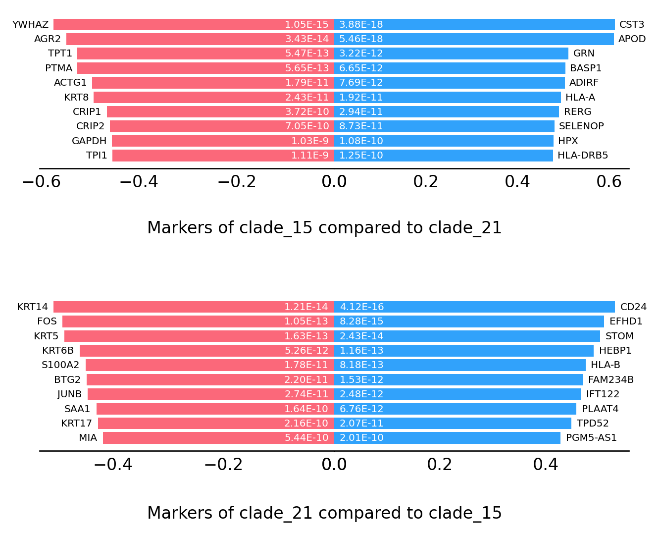
[18]:

st.spatial.trajectory.compare_transitions(data, trajectories=["clade_15", "clade_21"])

The result of comparison between clade_15 and clade_21 stored in 'adata.uns['compare_result']'

[19]:

st.pl.trajectory.DE_transition_plot(data)

../_images/tutorials_pseudotime_space_29_0.png

[19]:

AnnData object with n_obs × n_vars = 3798 × 22240
    obs: 'in_tissue', 'array_row', 'array_col', 'imagecol', 'imagerow', 'tile_path', 'louvain', 'louvain_anno', 'sub_cluster_labels', 'dpt_pseudotime'
    var: 'gene_ids', 'feature_types', 'genome', 'n_cells', 'mean', 'std'
    uns: 'spatial', 'log1p', 'pca', 'neighbors', 'louvain', 'louvain_colors', 'louvain_anno_colors', 'iroot', 'louvain_index_dict', 'paga', 'louvain_sizes', 'diffmap_evals', 'threshold_spots', 'split_node', 'global_graph', 'centroid_dict', 'available_paths', 'PTS_graph', 'clade_6', 'clade_15', 'clade_21', 'compare_result'
    obsm: 'spatial', 'X_pca', 'X_tile_feature', 'X_morphology', 'X_pca_morphology', 'X_diffmap'
    varm: 'PCs'
    layers: 'raw_count'
    obsp: 'distances', 'connectivities'

We also provide a function to compare the transition markers between two clades.