stSME Comparison

This tutorial shows the stSME normalization effect between of two scenarios:

• 1. normal (without stSME)

• 2. stSME applied on raw gene counts

In this tutorial we use Mouse Brain (Coronal) Visium dataset from 10x genomics website.

import scanpy as sc
import stlearn as st
import pathlib as pathlib

st.settings.set_figure_params(dpi=120)

# Ignore all warnings
import warnings

warnings.filterwarnings("ignore")

/Users/andrew/conda/stlearn/lib/python3.10/site-packages/louvain/__init__.py:54: UserWarning: pkg_resources is deprecated as an API. See https://setuptools.pypa.io/en/latest/pkg_resources.html. The pkg_resources package is slated for removal as early as 2025-11-30. Refrain from using this package or pin to Setuptools<81.
  from pkg_resources import get_distribution, DistributionNotFound
/Users/andrew/conda/stlearn/lib/python3.10/site-packages/stlearn/tl/cci/het.py:206: NumbaDeprecationWarning: The keyword argument 'nopython=False' was supplied. From Numba 0.59.0 the default is being changed to True and use of 'nopython=False' will raise a warning as the argument will have no effect. See https://numba.readthedocs.io/en/stable/reference/deprecation.html#deprecation-of-object-mode-fall-back-behaviour-when-using-jit for details.
  @jit(parallel=True, nopython=False)

st.settings.datasetdir =  pathlib.Path.cwd().parent / "data"

data = sc.datasets.visium_sge(sample_id="V1_Adult_Mouse_Brain")
data = st.convert_scanpy(data)

# pre-processing for gene count table
st.pp.filter_genes(data, min_cells=1)
st.pp.normalize_total(data)
st.pp.log1p(data)

Normalization step is finished in adata.X
Log transformation step is finished in adata.X

# pre-processing for spot image
st.pp.tiling(data, out_path="tiling")

# this step uses deep learning model to extract high-level features from tile images
# may need few minutes to be completed
st.pp.extract_feature(data)

Tiling image: 100%|███████████████████████████████████████████████████████████████████████████████████████████████████████████████████████████████████████████████████████████████████████████████████████████████████████████████████████████████████████████████████████████████████████████████████████ [ time left: 00:00 ]
Extract feature: 100%|███████████████████████████████████████████████████████████████████████████████████████████████████████████████████████████████████████████████████████████████████████████████████████████████████████████████████████████████████████████████████████████████████████████████████▉ [ time left: 00:00 ]

The morphology feature is added to adata.obsm['X_morphology']!

# run PCA for gene expression data
st.em.run_pca(data, n_comps=50)

PCA is done! Generated in adata.obsm['X_pca'], adata.uns['pca'] and adata.varm['PCs']

OMP: Info #276: omp_set_nested routine deprecated, please use omp_set_max_active_levels instead.

(1) normal (without stSME)

data_normal = data.copy()

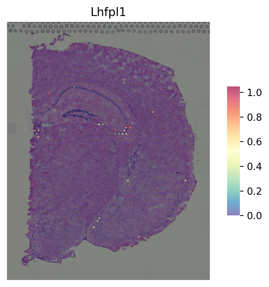
marker gene for CA3

i = "Lhfpl1"
st.pl.gene_plot(data_normal, gene_symbols=i, size=3)

AnnData object with n_obs × n_vars = 2702 × 21949
    obs: 'in_tissue', 'array_row', 'array_col', 'imagecol', 'imagerow', 'tile_path'
    var: 'gene_ids', 'feature_types', 'genome', 'n_cells'
    uns: 'spatial', 'log1p', 'pca'
    obsm: 'spatial', 'X_tile_feature', 'X_morphology', 'X_pca'
    varm: 'PCs'

marker gene for DG

i = "Pla2g2f"
st.pl.gene_plot(data_normal, gene_symbols=i, size=3)

AnnData object with n_obs × n_vars = 2702 × 21949
    obs: 'in_tissue', 'array_row', 'array_col', 'imagecol', 'imagerow', 'tile_path'
    var: 'gene_ids', 'feature_types', 'genome', 'n_cells'
    uns: 'spatial', 'log1p', 'pca'
    obsm: 'spatial', 'X_tile_feature', 'X_morphology', 'X_pca'
    varm: 'PCs'

(2) stSME applied on raw gene counts

data_SME = data.copy()
# apply stSME to normalise log transformed data
st.spatial.SME.SME_normalize(data_SME, use_data="raw")
data_SME.X = data_SME.obsm['raw_SME_normalized']
st.em.run_pca(data_SME, n_comps=50)

Adjusting data: 100%|█████████████████████████████████████████████████████████████████████████████████████████████████████████████████████████████████████████████████████████████████████████████████████████████████████████████████████████████████████████████████████████████████████████████████████ [ time left: 00:00 ]

The data adjusted by SME is added to adata.obsm['raw_SME_normalized']
PCA is done! Generated in adata.obsm['X_pca'], adata.uns['pca'] and adata.varm['PCs']

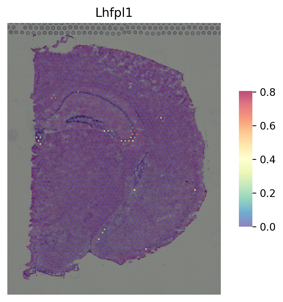
marker gene for CA3

i = "Lhfpl1"
st.pl.gene_plot(data_SME, gene_symbols=i, size=3)

AnnData object with n_obs × n_vars = 2702 × 21949
    obs: 'in_tissue', 'array_row', 'array_col', 'imagecol', 'imagerow', 'tile_path'
    var: 'gene_ids', 'feature_types', 'genome', 'n_cells'
    uns: 'spatial', 'log1p', 'pca', 'gene_expression_correlation', 'physical_distance', 'morphological_distance', 'weights_matrix_all', 'weights_matrix_pd_gd', 'weights_matrix_pd_md', 'weights_matrix_gd_md'
    obsm: 'spatial', 'X_tile_feature', 'X_morphology', 'X_pca', 'imputed_data', 'top_weights', 'raw_SME_normalized'
    varm: 'PCs'

marker gene for DG

i = "Pla2g2f"
st.pl.gene_plot(data_SME, gene_symbols=i, size=3)

AnnData object with n_obs × n_vars = 2702 × 21949
    obs: 'in_tissue', 'array_row', 'array_col', 'imagecol', 'imagerow', 'tile_path'
    var: 'gene_ids', 'feature_types', 'genome', 'n_cells'
    uns: 'spatial', 'log1p', 'pca', 'gene_expression_correlation', 'physical_distance', 'morphological_distance', 'weights_matrix_all', 'weights_matrix_pd_gd', 'weights_matrix_pd_md', 'weights_matrix_gd_md'
    obsm: 'spatial', 'X_tile_feature', 'X_morphology', 'X_pca', 'imputed_data', 'top_weights', 'raw_SME_normalized'
    varm: 'PCs'

Tutorial by Xiao Tan